


Courage to learn ML: Demystifying L1 & L2 Regularization
Comprehend the underlying purpose of L1 and L2 regularization


Welcome to the ‘Courage to learn ML’, where we kick off with an exploration of L1 and L2 regularization. This series aims to simplify complex machine learning concepts, presenting them as a relaxed and informative dialogue, much like the engaging style of “The Courage to Be Disliked,” but with a focus on ML.
These Q&A sessions are a reflection of my own learning path, which I’m excited to share with you. Think of this as a blog chronicling my journey into the depths of machine learning. Your interactions — likes, comments, and follows — go beyond just supporting; they’re the motivation that fuels the continuation of this series and my sharing process.
Today’s discussion goes beyond merely reviewing the formulas and properties of L1 and L2 regularization. We’re delving into the core reasons why these methods are used in machine learning. If you’re seeking to truly understand these concepts, you’re in the right place for some enlightening insights!
In this post, we’ll be answering the following questions:
What is regularization? Why we need it?
What is L1, L2 regularization?
What’s the reason behind the names L1 and L2 regularization?
How do we interpret the classic L1 and L2 regularization graph?
What are Lagrange multipliers, and how can we understand them intuitively?
Why are norms like L3 and L4 not commonly used?
Can L1 and L2 regularization be combined? And what are the advantages and disadvantages of doing this?
What is regularization? Why we need it?
Regularization is a cornerstone technique in machine learning, designed to prevent models from overfitting. Overfitting occurs when a model, often too complex, doesn’t just learn from the underlying patterns (signals) in the training data, but also picks up and amplifies the noise. This results in a model that performs well on training data but poorly on unseen data.
What is L1, L2 regularization?
There are multiple ways to prevent overfitting. L1, L2 regularization is mainly addresses overfitting by adding a penalty term on coefficients to the model’s loss function. This penalty discourages the model from assigning too much importance to any single feature (represented by large coefficients), thereby simplifying the model. In essence, regularization keeps the model balanced and focused on the true signal, enhancing its ability to generalize to unseen data.
Wait, why exactly do we impose a penalty on large weights in our models? How do large coefficients equate to increased model complexity?
While there are many combinations that can minimize the loss function, not all are equally good for generalization. Large coefficients tend to amplify both the useful information (signal) and the unwanted noise in the data. This amplification makes the model sensitive to small changes in the input, leading it to overemphasize noise. As a result, it cannot perform well on new, unseen data.
Smaller coefficients, on the other hand, help the model to focus on the more significant, broader patterns in the data, reducing its sensitivity to minor fluctuations. This approach promotes a better balance, allowing the model to generalize more effectively.
Consider an example where a neural network is trained to predict a cat’s weight. If one model has a coefficient of 10 and another a vastly larger one of 1000, their outputs for the next layer would be drastically different — 300 and 30000, respectively. The model with the larger coefficient is more prone to making extreme predictions. In cases where 30lbs is an outlier (which is quite unusual for a cat!), the second model with the larger coefficient would yield significantly less accurate results. This example illustrates the importance of moderating coefficients to avoid exaggerated responses to outliers in the data.
Could you elaborate on why there are multiple combinations of weights and biases in a neural network?
Imagine navigating the complex terrain of a neural network’s loss function, where your mission is to find the lowest point, or a ‘minima’. Here’s what you might encounter:

A Landscape of Multiple Destinations: As you traverse this landscape, you’ll notice it’s filled with various local minima, much like a non-convex terrain with many dips and valleys. This is because the loss function of a neural network with multiple hidden layers, is inherently non-convex. Each local minima represents a different combination of weights and biases, offering multiple potential solutions.
Various Routes to the Same Destination: The network’s non-linear activation functions enable it to form intricate patterns, approximating the real underlying function of the data. With several layers of these functions, there are numerous ways to represent the same truth, each way characterized by a distinct set of weights and biases. This is the redundancy in network design.
Flexibility in Sequence: Imagine altering the sequence of your journey, like swapping the order of biking and taking a bus, yet still arriving at the same destination. Relating this to a neural network with two hidden layers: if you double the weights and biases in the first layer and then halve them in the second layer, the final output remains unchanged. (Note this flexibility, however, mainly applies to activation functions with some linear characteristics, like ReLU, but not to others like sigmoid or tanh). This phenomenon is referred to as ‘scale symmetry’ in neural networks.
I’ve been reading about L1 and L2 regularization and observed that the penalty terms mainly focus on weights rather than biases. But why is that? Aren’t biases also coefficients that could be penalized?

In brief, the primary objective of regularization techniques like L1 and L2 is to predominantly prevent overfitting by regulating the magnitude of the model’s weights (personally, I think that’s why we call them regularizations). Conversely, biases have a relatively modest impact on model complexity, which typically renders the need to penalize them unnecessary.
To understand better, let’s look at what weights and biases do. Weights determine the importance of each feature in the model, affecting its complexity and the shape of its decision boundary in high-dimensional space. Think of them as the knobs that tweak the shape of the model’s decision-making process in a high-dimensional space, influencing how complex the model becomes.
Biases, however, serve a different purpose. They act like the intercept in a linear function, shifting the model’s output independently of the input features.
Here’s the key takeaway: Overfitting occurs mainly because of the intricate interplay between features, and these interactions are primarily handled by weights. To tackle this, we apply penalties to weights, adjusting how much importance each feature carries and how much information the model extracts from them. This, in turn, reshapes the model’s landscape and, as a result, its complexity.
In contrast, biases don’t significantly contribute to the model’s complexity. Moreover, they can adapt as weights change, reducing the need for separate bias penalties.
Why they call L1, l2 regularization?
The name, L1 and L2 regularization, comes from the concept of Lp norms directly. Lp norms represent different ways to calculate distances from a point to the origin in a space. For instance, the L1 norm, also known as Manhattan distance, calculates the distance using the absolute values of coordinates, like ∣x∣+∣y∣. On the other hand, the L2 norm, or Euclidean distance, calculates it as the square root of the sum of the squared values, which is sqrt(x² + y²)
In the context of regularization in machine learning, these norms are used to create penalty terms that are added to the loss function. You can think of Lp regularization as measuring the total distance of the model’s weights from the origin in a high-dimensional space. The choice of norm affects the nature of this penalty: the L1 norm tends to make some coefficients zero, effectively selecting more important features, while the L2 norm shrinks the coefficients towards zero, ensuring no single feature disproportionately influences the model.
Therefore, L1 and L2 regularization are named after these mathematical norms — L1 norm and L2 norm — due to the way they apply their respective distance calculations as penalties to the model’s weights. This helps in controlling overfitting.
I often come across the graph below when studying L1 and L2 regularization, but I find it quite challenging to interpret. Could you help clarify what it represents?
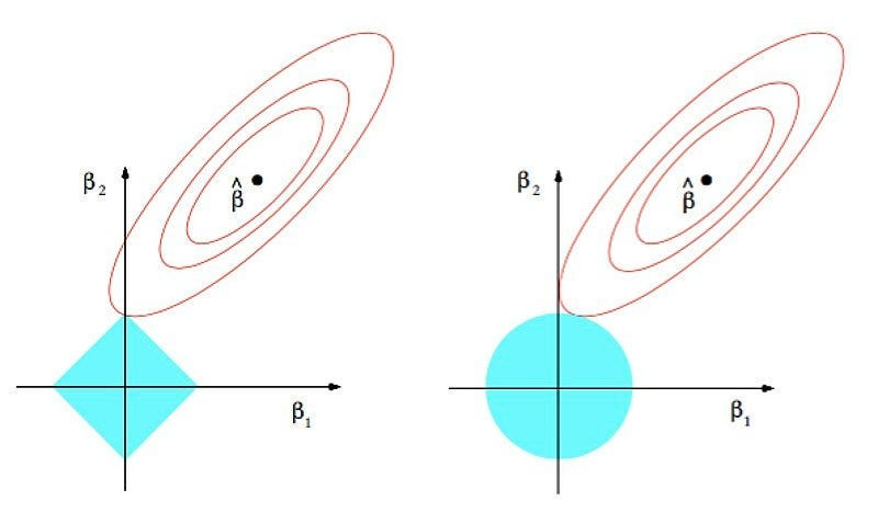
Alright, let’s unpack this graph step-by-step. To start, it’s essential to understand what its different elements signify. Imagine our loss function is defined by just two weights, w1 and w2 (in the graph we use beta instead of w, but they represent the same concept). The axes of the graph represent these weights we aim to optimize.
Without any weight penalties, our goal is to find w1 and w2 values that minimize our loss function. You can visualize this function’s landscape as a valley or basin, illustrated in the graph by the elliptical contours.
Now, let’s delve into the penalties. The L1 norm, shown as a diamond shape, essentially measures the Manhattan distance of w1 and w2 from the origin. The L2 norm forms a circle, representing the sum of squared weights.
The center of the elliptical contour indicates the global minimum of the objective function, where we find our ideal weights. The centers of the L1 and L2 shapes (diamond and circle) at the origin, where all weights are zero, highlight the minimal weight penalty scenario. As we increasing the penalty term’s intensity, the model’s weights would gravitate closer to zero. This graph is a visual guide to understanding these dynamics and the impact of penalties on the weights.
Understood. So…. The graph shows a dimension created by the weights, and the two distinct shapes illustrate the objective function and the penalty, respectively. How should we interpret the intersection point labeled w*? What does this point signify?
To understand the above graph as a whole, it’s essential to grasp the concept of Lagrange multipliers, a key tool in optimization. Lagrange multipliers aid in finding the optimal points (maximum or minimum) of a function within certain constraints.
Imagine you’re hiking up a mountain with the goal of reaching the peak. There are various paths, but due to safety, you’re required to stay on a designated safe path. Here, reaching the peak represents the optimization problem, and the safe path symbolizes the constraints.
Mathematically, suppose you have a function f(x, y) to optimize. This optimization must adhere to a constraint, represented by another function g(x, y) = 0.
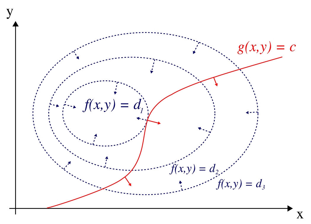
In the ‘Lagrange Multipliers 2D’ graph from Wikipedia, the blue contours represent f(x, y) (the mountain’s landscape), and the red curves indicate the constraints. The point where these two intersect, although not the peak point on the f(x, y) contour, represents the optimal solution under the given constraint. Lagrange multipliers solve this by merging the objective function with its constraints. In the other word, Lagrange multipliers will help you find the point easier.
So, if we circle back to that L1 and L2 graph, are you suggesting that the diamond and circle shapes represent constraints? And does that mean the spot where they intersect, that tangent point, is essentially the sweet spot for hitting the max of f(x, y) within those constraints?
Correct! The L1 and L2 regularization techniques can indeed be visualized as imposing constraints in the form of a diamond and a circle, respectively. So the graph helps us understand how these regularization methods impact the optimization of a function, typically the loss function in machine learning models.
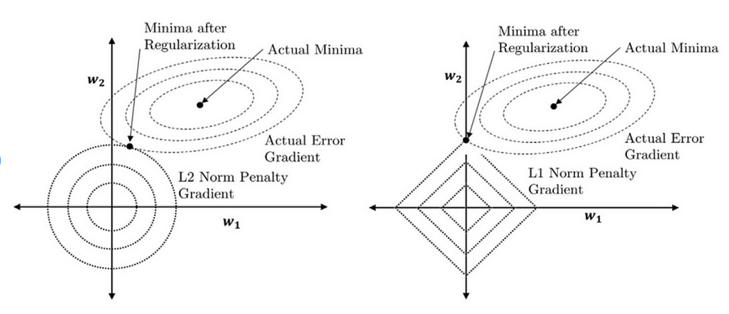
L1 Regularization (Diamond Shape): The L1 norm creates a diamond-shaped constraint. This shape is characterized by its sharp corners along the axes. When the optimization process (like gradient descent) seeks the point that minimizes the loss function while staying within this diamond, it’s more likely to hit these corners. At these corners, one of the weights (parameters of the model) becomes zero while others remain non-zero. This property of the L1 norm leads to sparsity in the model parameters, meaning some weights are exactly zero. This sparsity is useful for feature selection, as it effectively removes some features from the model.
L2 Regularization (Circle Shape): On the other hand, the L2 norm creates a circular-shaped constraint. The smooth, round nature of the circle means that the optimization process is less likely to find solutions at the axes where weights are zero. Instead, the L2 norm tends to shrink the weights uniformly without necessarily driving any to zero. This controls the model complexity by preventing weights from becoming too large, thereby helping to avoid overfitting. However, unlike the L1 norm, it doesn’t lead to sparsity in the model parameters.
I have a question based on our last discussion, I checked that for Lp norm, the value of p can be any number larger than 0. Why don’t use p between 0 and 1? What’s the reason behind not having an L0.5 regularization?
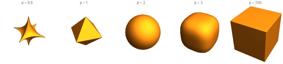
I’m glad you brought up this question. To get straight to the point, we typically avoid p values less than 1 because they lead to non-convex optimization problems. Let me illustrate this with an image showing the shape of Lp norms for different p values. Take a close look at when p=0.5; you’ll notice that the shape is decidedly non-convex.

This becomes even clearer when we look at a 3D representation, assuming we’re optimizing three weights. In this case, it’s evident that the problem isn’t convex, with numerous local minima appearing along the boundaries.
The reason why we typically avoid non-convex problems in machine learning is their complexity. With a convex problem, you’re guaranteed a global minimum — this makes it generally easier to solve. On the other hand, non-convex problems often come with multiple local minima and can be computationally intensive and unpredictable. It’s exactly these kinds of challenges we aim to sidestep in ML.
When we use techniques like Lagrange multipliers to optimize a function with certain constraints, it’s crucial that these constraints are convex functions. This ensures that adding them to the original problem doesn’t alter its fundamental properties, making it more difficult to solve. This aspect is critical; otherwise, adding constraints could add more difficulties to the original problem.
Why do we care about whether a problem or a constraint is a non-convex problem here? Aren’t most deep learning problems non-convex?
You questions touches an interesting aspect of deep learning. While it’s not that we prefer non-convex problems, it’s more accurate to say that we often encounter and have to deal with them in the field of deep learning. Here’s why:
Nature of Deep Learning Models leads to a non-convex loss surface: Most deep learning models, particularly neural networks with hidden layers, inherently have non-convex loss functions. This is due to the complex, non-linear transformations that occur within these models. The combination of these non-linearities and the high dimensionality of the parameter space typically results in a loss surface that is non-convex.
Local Minima are no longer a problem in deep learning: In high-dimensional spaces, which are typical in deep learning, local minima are not as problematic as they might be in lower-dimensional spaces. Research suggests that many of the local minima in deep learning are close in value to the global minimum. Moreover, saddle points — points where the gradient is zero but are neither maxima nor minima — are more common in such spaces and are a bigger challenge.
Advanced optimization techniques exist that are more effective in dealing with non-convex spaces. Advanced optimization techniques, such as stochastic gradient descent (SGD) and its variants, have been particularly effective in finding good solutions in these non-convex spaces. While these solutions might not be global minima, they often are good enough to achieve high performance on practical tasks.
Even though deep learning models are non-convex, they excel at capturing complex patterns and relationships in large datasets. Additionally, research into non-convex functions is continually progressing, enhancing our understanding. Looking ahead, there’s potential for us to handle non-convex problems more efficiently, with fewer concerns.
Why don’t we consider using higher norms, like L3 and L4, for regularization?
Recall the image we discussed earlier showing the shapes of Lp norms for various values of p. As p increases, the Lp norm’s shape evolves. For example, at p = 3, it resembles a square with rounded corners, and as p nears infinity, it forms a perfect square.
In our optimization problem’s context, consider higher norms like L3 or L4. Similar to L2 regularization, where the loss function and constraint contours intersect at rounded edges, these higher norms would encourage weights to approximate zero, just like L2 regularization. (If this part isn’t clear, feel free to revisit Part 2 for a more detailed explanation.) Based on this statement, we can talk about the two crucial reasons why L3 and L4 norms aren’t commonly used:
L3 and L4 norms demonstrate similar effects as L2, without offering significant new advantages (make weights close to 0). L1 regularization, in contrast, zeroes out weights and introduces sparsity, useful for feature selection.
Computational complexity is another vital aspect. Regularization affects the optimization process’s complexity. L3 and L4 norms are computationally heavier than L2, making them less feasible for most machine learning applications.
To sum up, while L3 and L4 norms could be used in theory, they don’t provide unique benefits over L1 or L2 regularization, and their computational inefficiency makes them less practical choice.
Is it possible to combine L1 and L2 regularization?
Yes, it is indeed possible to combine L1 and L2 regularization, a technique often referred to as Elastic Net regularization. This approach blends the properties of both L1 (lasso) and L2 (ridge) regularization together and can be useful while challenging.
Elastic Net regularization is a linear combination of the L1 and L2 regularization terms. It adds both the L1 and L2 norm to the loss function. So it has two parameters to be tuned, lambda1 and lambda2

What is the benefit of using Elastic Net regularization? If so, why don’t we use it more often?
By combining both regularization techniques, Elastic Net can improve the generalization capability of the model, reducing the risk of overfitting more effectively than using either L1 or L2 alone.
Let’s break it down its advantages:
Elastic Net provides more stability than L1. L1 regularization can lead to sparse models, which is useful for feature selection. But it can also be unstable in certain situations. For example, L1 regularization can select features arbitrarily among highly correlated variables (while make others’ coefficients become 0). While Elastic Net can distribute the weights more evenly among those variables.
L2 can be more stable than L1 regularization, but it doesn’t encourage sparsity. Elastic Net aims to balance these two aspects, potentially leading to more robust models.
However, Elastic Net regularization introduces an extra hyperparameter that demands meticulous tuning. Achieving the right balance between L1 and L2 regularization and optimal model performance involves increased computational effort. This added complexity is why it’s not frequently used.